Modeling porous electrodes: Part 3 (Newman’s BAND method)

I previously made a post about the basic formulation of porous electrode theory (part 1), and a post about how the choice of kinetic expression determines what the result will look like (part 2). The purpose of this post is to explain how to solve these basic problems using the BAND formulation found in John Newman’s textbook Electrochemical Systems (Newman and Thomas-Alyea in the Third Edition). I also provide Python code so you can get the solution yourself and modify it for your own teaching and learning needs.

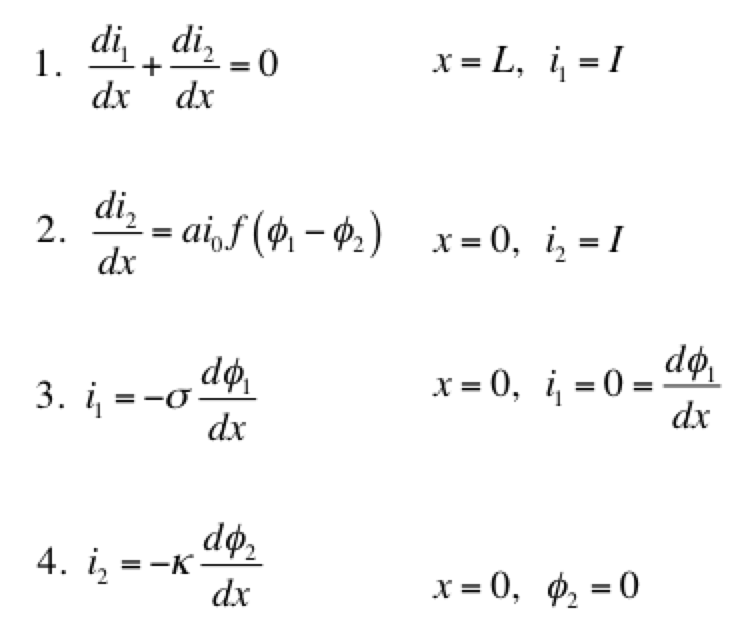
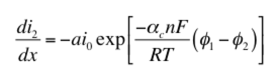
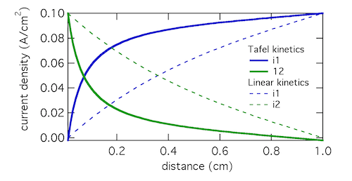
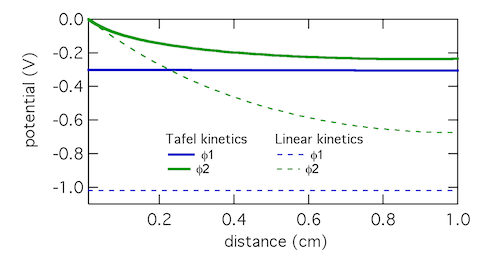
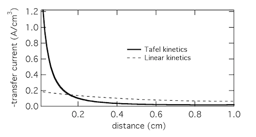
As a model problem we’ll use the boundary value problem of Tafel kinetics in a concentration-independent porous electrode in Cartesian coordinates. The reason to choose this one is because Newman and Tobias provide the analytical solution in their 1962 paper “Theoretical Analysis of Current Distribution in Porous Electrodes.” You can also find this solution in Fuller and Harb’s Electrochemical Engineering, in the problems at the end of Chapter 5. The reason to choose a problem with an analytical solution is so you can check your work to know if it’s right! We lay out the problem below, which is the same as that in Newman and Tobias (1962) except one sign convention. This is four equations with four unknowns (i1, i2, Φ1, Φ2):

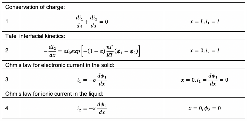
If you read the electrochemical engineering literature, solving problems such as this with Newman’s BAND method often comes up, and you might wonder what that is. Technically “BAND” is some Fortran code set up to solve 2-point boundary value problems in a way that is convenient for electrochemists. (My own favorite document written about BAND is “Modeling and reactor simulation” by Douglas Bennion in the AIChE symposium series 1983, Vol 79, Num 229, pp 25-36. It’s a resource meant for teachers and is somewhat hard to find so I’ve uploaded it here.) The formulation Newman uses to set up the problem casts each of the equations in this way:

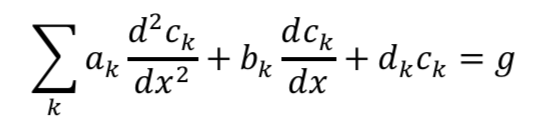
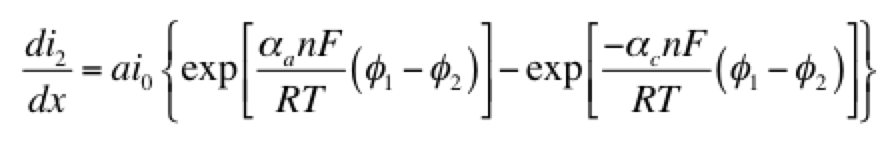
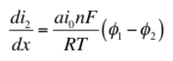
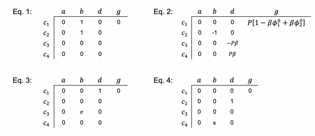
Here c is a variable. The coefficients a, b, and d are those for the second derivative, first derivative, and the variable itself. And g is the constant term. When you linearize equation 2 above and then cast all of the four equations this way, you get something that looks like the tables below. I’ve collected some constants together as ß and P to keep it from looking too messy:

Once you have this, you can (a) build a block tridiagonal matrix, (b) choose initial guesses for the answers, and (c) iterate to a solution by repeatedly solving the problem until your initial guesses and final answers match. Explaining how this works is too long for a blog post, so follow these links for:

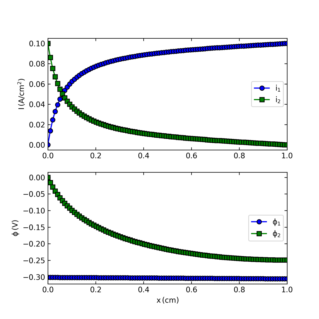
If you execute the code you should get a figure like that below, which solves the problem. (I still use Python 2.7 so you might have to do some mild editing and debugging.)

What I use this for

The reason I started writing a BAND-type method in Python is (1) I wanted to learn more about how BAND worked so I could teach it better, and (2) I wanted to model electrochemical systems without having to buy expensive software or use Fortran. It’s not exactly like Newman’s code, which also included a function to solve the matrix problem. Rather, this code lets you input the problem in Newman’s way and build the corresponding block tridiagonal matrix, then it uses SciPy to solve the matrix problem.

When I was working on the paper above in 2016, I wanted to compare experimental data to the Chen + Podlaha + Cheh alkaline battery model developed in the 1990s. Python seems like the best choice for something you can also develop as a teaching tool, so I used that to generate the results in Figure 3 of the paper. Since then I’ve used it to train some MS students getting insight into shallow-cycled MnO2 cathodes. When Zhicheng Lu’s MS thesis appeared on the internet, I received a few questions about the model by email. So this post is meant to help anyone doing similar things.

Lead pipe corrosion in Flint

There’s a wonderful paper by Olson et al. in Environmental Science & Technology Letters called Forensic Estimates of Lead Release from Lead Service Lines during the Water Crisis in Flint, Michigan. From the abstract:

The findings provide evidence that selective dissolution of lead phosphate minerals occurred because of the absence of orthophosphate during the crisis.

I’m teaching the chemical engineering intro class at Northeastern this semester, and I’m putting in some information from this paper. Mismanagement of the water supply in Flint is a pretty perfect example of how not to do chemical engineering. The piping infrastructure in Flint required orthophosphate treatment of the water, and for some reason this practice was stopped.

The direction of change

It’s been a busy summer, and we’ve got a few exciting battery-related surprises coming up soon at the CUNY Energy Institute. This week I’m getting ready for the start of my Transport Phenomena I class at NYU. Transport phenomena is about understanding and describing all physical changes you may find in the world.

Over the course of the year I show the class the following transport equations, which are my favorite parts of the class. Realizing these equations, which are all basically statements of the second law of thermodynamics, have a common origin is the philosophically most fun thing about studying transport.

Fourier’s law states that heat flows down a temperature gradient (with proportionality constant k, the thermal conductivity):

fouriers law

Fick’s law tells you mass moves from areas of high concentration to low:

ficks law

Ohm’s law states that current moves down a potential gradient (and so electrons move up the gradient due to the dyslexic way current is defined):

ohms law

And Newton’s law of viscosity (which is a little more complicated-looking due to the way fluids can change their density) tells you momentum transports from locations of high velocity to low.

newtons law of visc

The negative signs in these equations are the second law of thermodynamics. Those negative signs are a consequence of the fact that the universe tends towards states of higher entropy or higher probability. Of course you can make heat flow up a temperature gradient using, for example, an air conditioner. But that requires a machine, which is what you learn in a thermodynamics class. And that’s what separates “transport” from “thermo” for a chemical engineering student.


Dimensional analysis of batteries

Now that high performance batteries are a big part of our daily lives, powering our cell phones and portable computers, we naturally want to spend less time waiting for batteries to charge up. This has prompted the search for ultrafast batteries. We would like batteries that can cycle at high currents, either discharging or charging in no time. Perhaps you’d like to charge your cell phone in under a minute, or you’d like to charge your EV in the same few minutes it takes to fill up with gasoline.

Either way, fast batteries are an engineering challenge. A good way to think of this is that it’s fairly easy to make a small battery that can cycle rapidly, but as a battery becomes larger, approaching the size it takes to power your phone or car, it gets more challenging. The way to understand this is to look at dimensional analysis.

Dimensional analysis example

Dimensional analysis is the engineering concept used to understand the scale or size of something, and was discovered by Galileo. Basically, to make size not matter, you have to eliminate all dimensionality in a problem. To do this you multiply/divide the important constants in the problem to make the dimensions cancel out.

Up above is a dimensionless number for a structure, which involves: the yield strength and density of the structure materials, the gravitational constant (gravity pulls down on the structure), and the structure size, which is L, a length like the height. Consider this: is a matchstick model of Notre Dame Cathedral a fair model of the real Notre Dame cathedral? And if so, does it mean you could make the real Cathedral out of wood too?

The answer is no. The matchstick model is not at all like the real Cathedral, because while size does change between the two, gravity does not. A successful matchstick model means you could build the real Cathedral out of wood … only on a smaller planet with a lower value of g.

Dimensional analysis of a battery

Dimensional analysis of a battery is similar to that of the Cathedral above. Imagine a small research-scale battery you might work with in a lab, and then imagine a practical battery based on it. The practical battery has been developed and scaled-up to provide the power and energy required by the application. Scaling up a battery almost always involves thickening the electrodes, and we will call this “increasing L.” The important length scale of an electrode is usually the thickness in the same dimension as current flow.

I’ve written previously about reaction rate distributions in battery electrodes (here and here). The dimensionless number δ (or John Newman’s number) tells you how balanced the reactions in a battery electrode are. When L increases, it tells you that something else has to decrease, like current I, if you want to keep δ the same. This means in general a small battery will charge fast and a large battery will charge slowly.

This is unless the other parameters in δ change accordingly to keep behavior the same … for example the porosity could be increased and that would increase the pore conductivity or κ and therefore decrease δ. But usually this goes in the opposite direction: as you scale up typically you want to achieve higher active material loading, pushing you to decrease porosity and thus decrease κ and increase δ. In fact, almost every decision you make during scale-up forces you to increase δ overall.

For this reason, the very first research decision you should try to make is to set L at the same value in your small battery that you will need in the final device. That way it becomes easier to understand scale-up, and you can extrapolate research results to real-world situations. When analyzing a fast battery, first check L and see whether scale-up will require it to increase.

Modeling porous electrodes: Part 2

A secondary current distribution model considers:

  1. Ohm’s law resistance, and
  2. kinetic charge-transfer resistance

while resistance related to concentration variations is ignored. Beginning with the equations given in Modeling porous electrodes: Part 1, the following can be written:

Porous 2 equations

Eq 1 is conservation of charge; Eq 2 is some expression of electrochemical reaction kinetics; and Eqs 3 & 4 are Ohm’s law for the solid and liquid phases. The boundary conditions are such that a current density of I is being produced by the electrode. The liquid phase potential φ2 is arbitrarily set to 0 V at x = 0. The specific expression for the electrode kinetics (Eq 2) needs to be specified. The concentration-independent Butler-Volmer expression can be used:

Porous-2-Butler-Volmer.png

The left hand side of this expression is the transfer current, with units of A/cm3, and gives the amount of electrochemical reaction occurring at any point. The right hand side has two components: the anodic and cathodic kinetic terms. The downside of the Butler-Volmer equation is its complexity. Finding an analytical solution to the above set of differential equations requires a more simplified kinetic expression. One possible simplification is to assume the overpotential (φ– φ2) is highly negative. This means only the cathodic term in the Butler-Volmer equation need be considered:

Porous-2-Tafel

The right hand side of this expression is a form of the Tafel equation. (An analogous anodic form can be used when overpotential is highly positive.) Another possible simplification is to assume the overpotential (φ1 – φ2) is small. In this case both anodic and cathodic terms are important. Substituting the first two terms of a Taylor series for the exponentials results in:

Porous-2-linear

This linear kinetic expression is valid only at low currents. Which approximation of the kinetic expression is appropriate depends on the conditions of interest. Choosing the following values for physical parameters:

  • electrode area per volume, a = 23,300 cm-1
  • transfer coefficients, αaαc = 0.5
  • exchange current density, i0 = 2 x 10⁻⁷ A/cm2
  • current density, I = 0.1 A/cm2
  • length, L = 1 cm
  • electrolyte conductivity, κ = 0.06 S/cm
  • electrode conductivity, σ = 20 S/cm

we assume that the Tafel approximation for kinetics will be valid, because the current density is much larger than the exchange current density. Solving the set of equations 1-4 for both Tafel and linear kinetics gives the results below:

 Porous electrode current

Porous electrode potential

The Tafel kinetic expression predicts that current exchange from liquid to solid phases (ionic current to electronic current) will be concentrated near x = 0, the location closest to the counter electrode. There (φ1 – φ2) will be near 300 mV, falling away further into the electrode. In contrast, the linear kinetic expression predicts a more even exchange of current through the electrode, and much higher values of (φ1 – φ2). This is because the linear expression is a softer function of overpotential than the exponential one. The Tafel approximation is clearly the more appropriate in this case because (φ1 – φ2) » RT/F which is 25.7 mV at room temperature.

2015-03-04 taf-lin trans

Plotting the transfer current di2/dx shows that in reality the electrochemical reaction is concentrated in the front 10% of the electrode. Linear kinetics tend to result in more uniform current distributions, but for this to be the case i0 > I will need to hold.

Click here for Modeling porous electrodes: Part 3, which is about solving porous electrode problems using Newman’s BAND method.