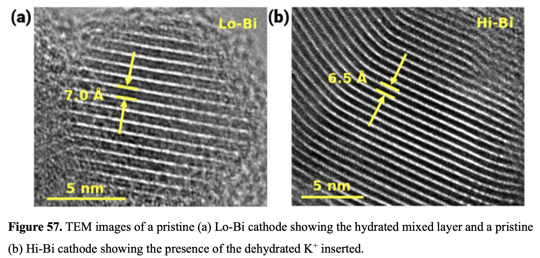
Cylindrical alkaline batteries: Pulsed vs. continuous discharge

We have a new paper out in The Journal of Power Sources, which is a collaboration with Energizer. We use high energy white beam tomography to study the distribution of ZnO in the anodes of cylindrical alkaline batteries. (These are AAA, but we also studied AA sizes.) The finding is that the distribution of ZnO is a strong function of how the battery was discharged. In the image below, batteries (d) and (e) were discharged to the same depth (295 mAh) at the same rate (21 mA).

Continuous discharge (e) matched what you expect from a computational battery model: relatively dense ZnO (pink) found mostly near the separator, around the anode’s circumference. However, if the discharge was pulsed (d), the ZnO had a very low density (blue) and was mostly in large clumps in the anode interior. Since most primary batteries are used in an intermittent or pulsed manner, understanding how this affects where the resistive ZnO is located is important for getting more capacity out of the cells. We found that varying the ZnO density helps reconcile computational models with experimental results.

PhD student Dom Guida came up with a custom segmentation method to analyze these data. All the details are in the paper and the supplemental info. This tomography was special because the resolution was good (a little less than 3 microns) with a quite large field of view, letting us use unaltered AA and AAA cells and record the entire battery diameter.

Space-filling shapes in composite solid electrolyte (CSE) batteries

We have a new paper in The Journal of Physical Chemistry C, written by Dr. Bebi Patil. It deals with composite solid electrolytes (CSEs) based on (1) a Li-conducting filler (LATP) in (2) a polymer matrix (PEO + LiTFSI). This work demonstrates that engineering fillers to have space-filling shapes has a profound positive impact on conductivity of the resulting CSE. Our approach was to engineer a micron-scale filler with a hollow-sphere morphology (shown below) because hollow spheres fill space efficiently and shift agglomeration to the level of the secondary particles. Also the hollow spheres are porous and have both an inner and outer surface.

With CSEs, it is of paramount importance for the ceramic filler to present maximum surface area to the polymer matrix. This is typically done by exploiting the high surface area to volume ratio of nanomaterials. To achieve a percolated Li-conducting interphase across the electrolyte, many groups have engineered fillers in a nanofiber or nanorod morphology. However, our micron-scale hollow sphere material performed as well as or better than nanoscale materials. It had a near-record room temperature conductivity (1.64 × 10⁻⁴ S/cm) for a PEO/LATP-based CSE. (This is a good start, but conductivity still needs to be higher for CSEs to be widely used in battery products.)

Li metal batteries based on CSEs are desired because polymer processing would be simpler to integrate into battery manufacturing than the high temperature methods required for ceramic solid electrolytes. Also, polymers make good interfaces with battery active materials. The challenge is that their Li conductivities are generally much lower than other solid electrolytes (like sulfides or garnets). Including a filler material improves the conductivity. There are several reasons for this, some of which are not completely understood.

Northeastern student Marisol Chang Zapata designed us a wonderful cover image!

Bi Enables the Formation of Disordered Birnessite in Rechargeable Alkaline Batteries

We have a new paper out in the Journal of the Electrochemical Society, written by Andrea Bruck. It continues our work on full 617 mAh/g rechargeability of MnO2 in alkaline batteries. Getting that full capacity reversibly enables a design pathway to get very inexpensive ($50/kWh) and high energy density (200 Wh/L) aqueous electrolyte rechargeable Zn-MnO2 batteries for the power grid. Aqueous electrolytes are desirable as an alternative to Li-ion batteries, which have flammable electrolytes, and become more of a safety risk at large scales.

Our main finding is the identification of an amorphous or “disordered” intermediate species during cycling. The figure above shows the voltage profile of the MnO2 cathode during cycling, and each section is labeled with the major material compound that is formed during that stage. (The discharge stages are labeled d1, d2, and d3. Likewise the charging stages are c1, c2, and c3.) We mix the MnO2 with bismuth oxide or Bi2O3, which is what makes it rechargeable. And during step c2, we have demonstrated a disordered compound we had never seen before. The reason we had never seen it is because all the other compounds are crystalline, and crystalline things are very easy to see. Disordered (or non-crystalline) things are often more challenging to put your finger on.

The figure above shows the structure of the layered birnessite or ẟ-MnO2, which consists of [MnO6] slabs separated by an interlayer. This data is from X-ray diffraction (XRD), which uses long-range crystallinity to produce a material fingerprint. This fingerprint is in the form of peaks or reflections, and the plot has the experimental data (black) compared to a theoretical calculation (red). We used a method called Rietveld refinement to match these and get the coordinates for all of the atoms in the material. (For example, we can tell the birnessite is hexagonal and the slab-to-slab distance is 7.131 Å)

However, you can’t observe a material by XRD if it doesn’t have good crystallinity, a.k.a. the “long-range order” to diffract X-rays. Instead we used operando Raman spectroscopy, which fingerprints materials using their response to a laser. Birnessite materials result in a series of Raman vibrational bands, the largest of which are ν1 and ν2. The figure above shows the Raman spectrum during the charge step both without Bi (top) and with Bi (bottom). In the top plots, the ν1 and ν2 bands didn’t appear until the blue dot, which is the c3 stage. However, with Bi, they appeared very early, even before the red dot, which is in the c2 stage. We know this is a disordered birnessite because it was not visible to XRD, but showed up clearly with Raman spectroscopy.

This is exciting because no one really knows why Bi makes birnessite rechargeable. Since we see it enables this formation of a disordered birnessite, that could be the key.

EDXRD review paper

We have a new paper out, which is a review paper on using energy dispersive X-ray diffraction (EDXRD) for battery characterization. EDXRD had previously been used to get crystallography data from inside diamond anvil cells, and also from the bulk interior of engineering materials like turbine blades. Using it to look inside sealed batteries was a good idea. It wasn’t my idea, but I’m one of the battery people they found to try it. I have a passion for current distributions, and EDXRD is a wonderful way to directly observe current distributions.

The paper was written with Amy Marschilok and the Takeuchi group at Stony Brook, and also with Mark Croft at Rutgers. We’re still using EDXRD to watch complex mechanisms inside batteries (without the fear that opening the battery will change anything), but since the review paper spans 2012-2020, it was a good idea to catalog past work in one place. The new HEX beamline under development at NSLS-II will be the premier EDXRD resource sometime soon. The figure below is an attempt to explain what exactly EDXRD gets you (atomic scale information, as a function of the electrode scale) and why it’s important (look how thick that electrode is). If you ever want to talk about EDXRD drop me a line.

Modeling porous electrodes: Part 3 (Newman’s BAND method)

I previously made a post about the basic formulation of porous electrode theory (part 1), and a post about how the choice of kinetic expression determines what the result will look like (part 2). The purpose of this post is to explain how to solve these basic problems using the BAND formulation found in John Newman’s textbook Electrochemical Systems (Newman and Thomas-Alyea in the Third Edition). I also provide Python code so you can get the solution yourself and modify it for your own teaching and learning needs.

As a model problem we’ll use the boundary value problem of Tafel kinetics in a concentration-independent porous electrode in Cartesian coordinates. The reason to choose this one is because Newman and Tobias provide the analytical solution in their 1962 paper “Theoretical Analysis of Current Distribution in Porous Electrodes.” You can also find this solution in Fuller and Harb’s Electrochemical Engineering, in the problems at the end of Chapter 5. The reason to choose a problem with an analytical solution is so you can check your work to know if it’s right! We lay out the problem below, which is the same as that in Newman and Tobias (1962) except one sign convention. This is four equations with four unknowns (i1, i2, Φ1, Φ2):

If you read the electrochemical engineering literature, solving problems such as this with Newman’s BAND method often comes up, and you might wonder what that is. Technically “BAND” is some Fortran code set up to solve 2-point boundary value problems in a way that is convenient for electrochemists. (My own favorite document written about BAND is “Modeling and reactor simulation” by Douglas Bennion in the AIChE symposium series 1983, Vol 79, Num 229, pp 25-36. It’s a resource meant for teachers and is somewhat hard to find so I’ve uploaded it here.) The formulation Newman uses to set up the problem casts each of the equations in this way:

Here c is a variable. The coefficients a, b, and d are those for the second derivative, first derivative, and the variable itself. And g is the constant term. When you linearize equation 2 above and then cast all of the four equations this way, you get something that looks like the tables below. I’ve collected some constants together as ß and P to keep it from looking too messy:

Once you have this, you can (a) build a block tridiagonal matrix, (b) choose initial guesses for the answers, and (c) iterate to a solution by repeatedly solving the problem until your initial guesses and final answers match. Explaining how this works is too long for a blog post, so follow these links for:

If you execute the code you should get a figure like that below, which solves the problem. (I still use Python 2.7 so you might have to do some mild editing and debugging.)

What I use this for

The reason I started writing a BAND-type method in Python is (1) I wanted to learn more about how BAND worked so I could teach it better, and (2) I wanted to model electrochemical systems without having to buy expensive software or use Fortran. It’s not exactly like Newman’s code, which also included a function to solve the matrix problem. Rather, this code lets you input the problem in Newman’s way and build the corresponding block tridiagonal matrix, then it uses SciPy to solve the matrix problem.

When I was working on the paper above in 2016, I wanted to compare experimental data to the Chen + Podlaha + Cheh alkaline battery model developed in the 1990s. Python seems like the best choice for something you can also develop as a teaching tool, so I used that to generate the results in Figure 3 of the paper. Since then I’ve used it to train some MS students getting insight into shallow-cycled MnO2 cathodes. When Zhicheng Lu’s MS thesis appeared on the internet, I received a few questions about the model by email. So this post is meant to help anyone doing similar things.