We have a new paper out in the Journal of the Electrochemical Society, written by Andrea Bruck. It continues our work on full 617 mAh/g rechargeability of MnO₂ in alkaline batteries. Getting that full capacity reversibly enables a design pathway to get very inexpensive ($50/kWh) and high energy density (200 Wh/L) aqueous electrolyte rechargeable Zn-MnO₂ batteries for the power grid. Aqueous electrolytes are desirable as an alternative to Li-ion batteries, which have flammable electrolytes, and become more of a safety risk at large scales.

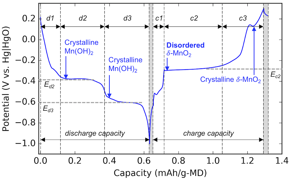
Our main finding is the identification of an amorphous or “disordered” intermediate species during cycling. The figure above shows the voltage profile of the MnO₂ cathode during cycling, and each section is labeled with the major material compound that is formed during that stage. (The discharge stages are labeled d1, d2, and d3. Likewise the charging stages are c1, c2, and c3.) We mix the MnO₂ with bismuth oxide or Bi₂O₃, which is what makes it rechargeable. And during step c2, we have demonstrated a disordered compound we had never seen before. The reason we had never seen it is because all the other compounds are crystalline, and crystalline things are very easy to see. Disordered (or non-crystalline) things are often more challenging to put your finger on.

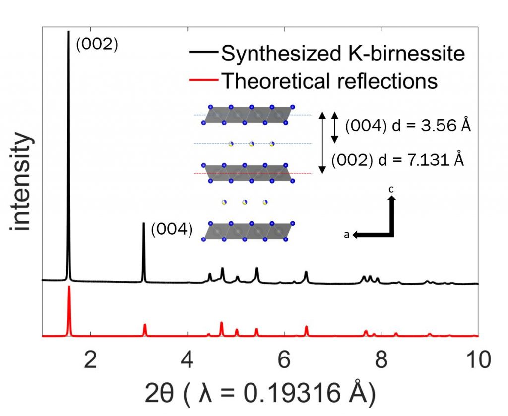
The figure above shows the structure of the layered birnessite or ẟ-MnO₂, which consists of [MnO₆] slabs separated by an interlayer. This data is from X-ray diffraction (XRD), which uses long-range crystallinity to produce a material fingerprint. This fingerprint is in the form of peaks or reflections, and the plot has the experimental data (black) compared to a theoretical calculation (red). We used a method called Rietveld refinement to match these and get the coordinates for all of the atoms in the material. (For example, we can tell the birnessite is hexagonal and the slab-to-slab distance is 7.131 Å)

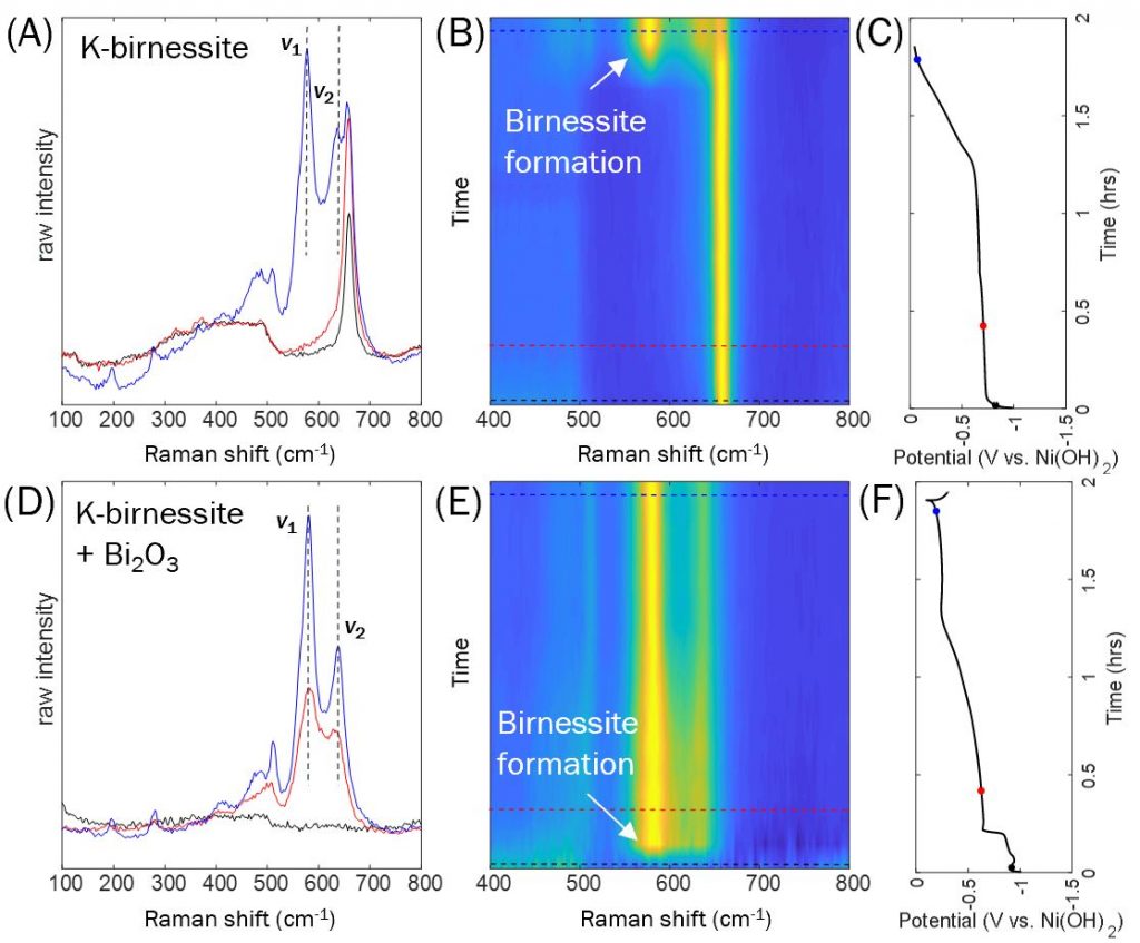
However, you can’t observe a material by XRD if it doesn’t have good crystallinity, a.k.a. the “long-range order” to diffract X-rays. Instead we used operando Raman spectroscopy, which fingerprints materials using their response to a laser. Birnessite materials result in a series of Raman vibrational bands, the largest of which are ν₁ and ν₂. The figure above shows the Raman spectrum during the charge step both without Bi (top) and with Bi (bottom). In the top plots, the ν₁ and ν₂ bands didn’t appear until the blue dot, which is the c3 stage. However, with Bi, they appeared very early, even before the red dot, which is in the c2 stage. We know this is a disordered birnessite because it was not visible to XRD, but showed up clearly with Raman spectroscopy.

This is exciting because no one really knows why Bi makes birnessite rechargeable. Since we see it enables this formation of a disordered birnessite, that could be the key.